HomeOptimal trajectory generation for autonomous vehicles
Autonomous driving · Motion planning
Optimal trajectory generation for autonomous vehicles
From Frenét polynomial sampling to nonlinear optimization
An autonomous driving stack needs trajectories that are collision-free, kinematically feasible, and comfortable — and they must be replanned every cycle (on the order of 100 ms). This line of work follows that requirement through three motion planners: Werling-style jerk-optimal polynomial sampling in a Frenét frame; piecewise-jerk quadratic programs that solve for path and speed directly in Frenét while encoding object decisions such as left/right nudge, overtake, or yield; and a nonlinear program that computes trajectories for complex static-obstacle avoidance in Cartesian space.
Existing work: Werling polynomial sampling
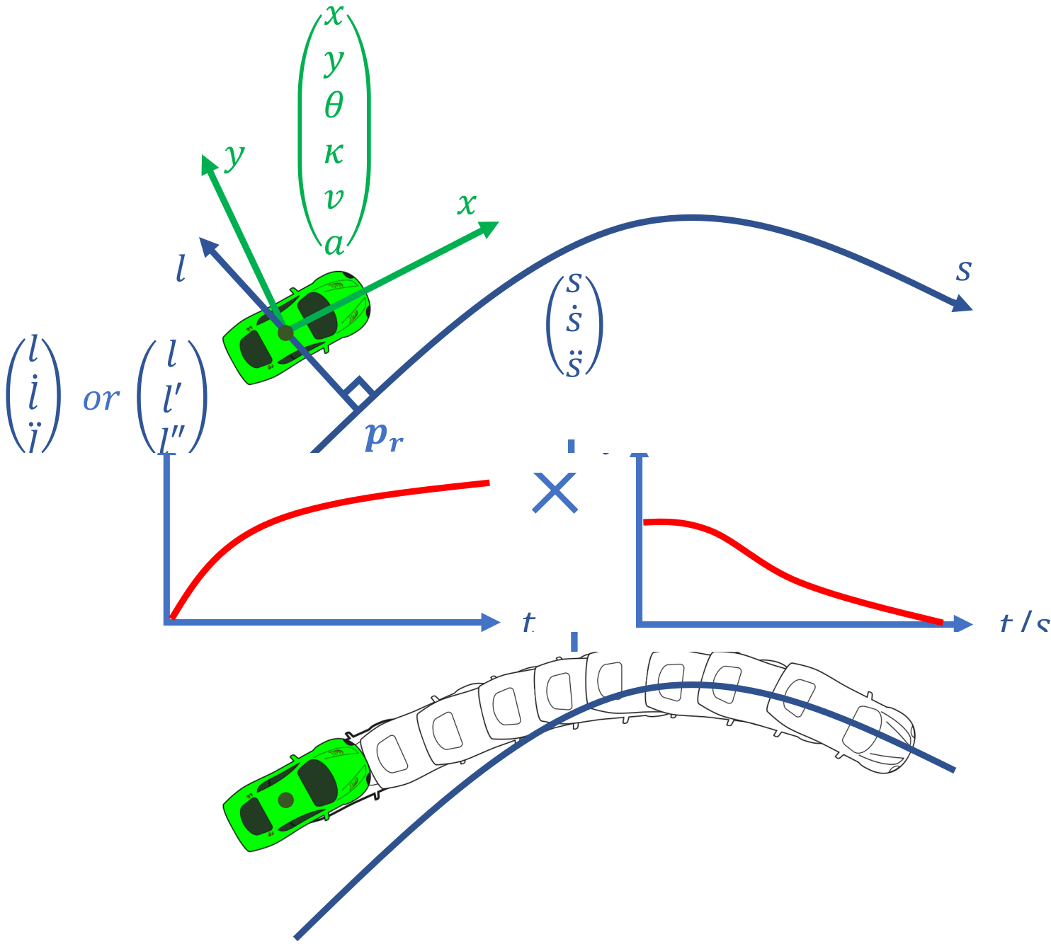
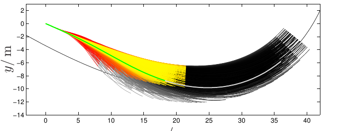
A foundational planner is Werling et al. (ICRA 2010). Motion along a road center line is decoupled into two independent 1-D problems in a Frenét frame: lateral motion perpendicular to the center line, and longitudinal motion along it. Quintic and quartic polynomials are then sampled by varying end conditions and parameters to produce candidate 1-D motions. Lateral and longitudinal candidates are paired, transformed back to the map frame, collision-checked, and scored; the best valid combination is selected each replan cycle.
The idea is straightforward and works well in simple driving environments.
The limits show up quickly in complex urban scenes: a single polynomial has few degrees of freedom and cannot represent the trajectories those scenes need, and sampling without regard to constraints becomes extremely inefficient.
Piecewise-jerk framework
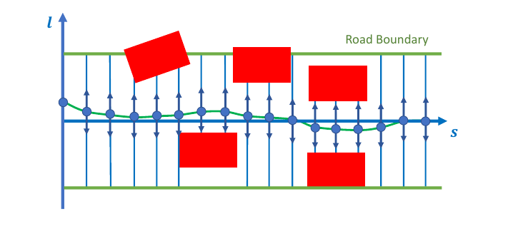
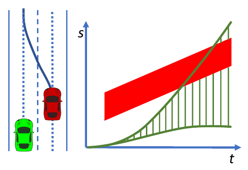
Piecewise-jerk planning replaces polynomial sampling with direct optimization. Each 1-D motion is a sequence of knots — position, velocity, and acceleration — with consecutive knots joined by a constant jerk. Those jerk terms act as control variables that reshape the motion, yielding a profile that is globally flexible and locally second-order smooth. A quadratic program (QP) then finds the optimum inside a homotopy corridor.
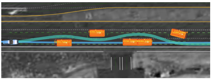
Applied longitudinally as s(t) (IEEE ITSC 2019), the same recipe plans speed along a smoothed guide line under centripetal acceleration limits, with dynamic constraints entering through a path–time obstacle graph. Applied laterally as l(s) (IEEE IV 2020; Baidu Apollo Open Platform), it plans a path inside a corridor built from the guide line, road bounds, and static obstacles.
Together they form a hierarchical path-then-speed stack that solves for geometry and speed directly — dense enough for cluttered static scenes, and fast enough for onboard replanning.
Nonlinear optimization
Piecewise-jerk planning in Frenét still has structural limits. Map-frame kinematics — curvature, curvature rate, bicycle-model feasibility — become awkward after the frame transform and are often enforced only approximately. Accurate decoupling also needs a highly smooth guide line with C³ continuity; because comfort is measured relative to that line, poor guide-line geometry produces poor trajectories.
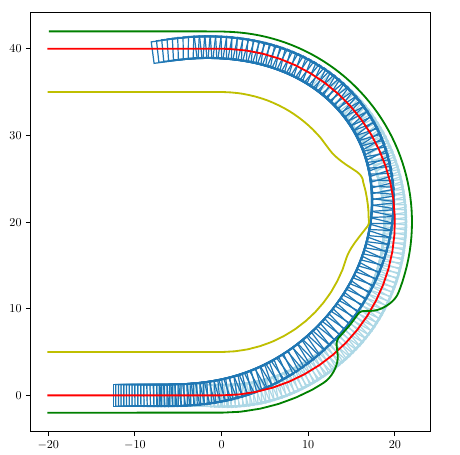
The later planner (arXiv 2023) keeps the hierarchical path/speed split, but solves static-obstacle avoidance as a nonlinear program in the map frame. A trajectory is a sequence of discretized vehicle states (position, heading, curvature, speed, acceleration); the optimizer searches over jerks and curvature rates while enforcing kinematic equalities between consecutive states.
Engineering keeps it onboard: warm starts from the previous cycle, corridor smoothing that reuses the earlier QP smoother lineage, and fast projection for collision checks. A 6-second horizon solves in about 10 ms on an Intel i7 and about 20 ms on one Nvidia Drive Orin core.
Some design principles from past lessons
- Drop heavy dependence on a high-quality reference (guide) line for Frenét planning. If the planner only works when that line is already smooth, well placed, and C³-clean, the hard problem has been pushed upstream rather than solved.
- Stop relying on a human-designed geometry or speed profile as a soft target the planner must track. The motion planner should be self-contained — producing feasible, comfortable trajectories from map, obstacles, and vehicle limits — instead of following hand-tuned path or speed references.
- Prefer strict constraint satisfaction. Soft penalties and approximate bounds hide failures until they show up on the road; hard feasibility is the contract worth keeping.
- Choose a representation at one of the extremes: a single closed-form polynomial, or a fully discretized trajectory (piecewise-jerk, later NLP). Avoid piecewise-polynomial splines — they sit in a half-measure middle ground that is neither fast nor easy to control.
- Joint geometry and speed planning looks appealing in theory, but in practice it adds coupling and tuning without enough operational payoff. Prefer keeping path and speed separable.
Keywords
Frenét frame · Quadratic programming · Nonlinear optimization · Vehicle kinematic model · Ipopt